When I checked my results on th website, I came across the dataset of the preliminary results, and I was pleased to see that these results included not only the final time of all runners, but also their mid-race results. I was at the top of the hill after 40 min and it took me 1h21 to run the whole race.
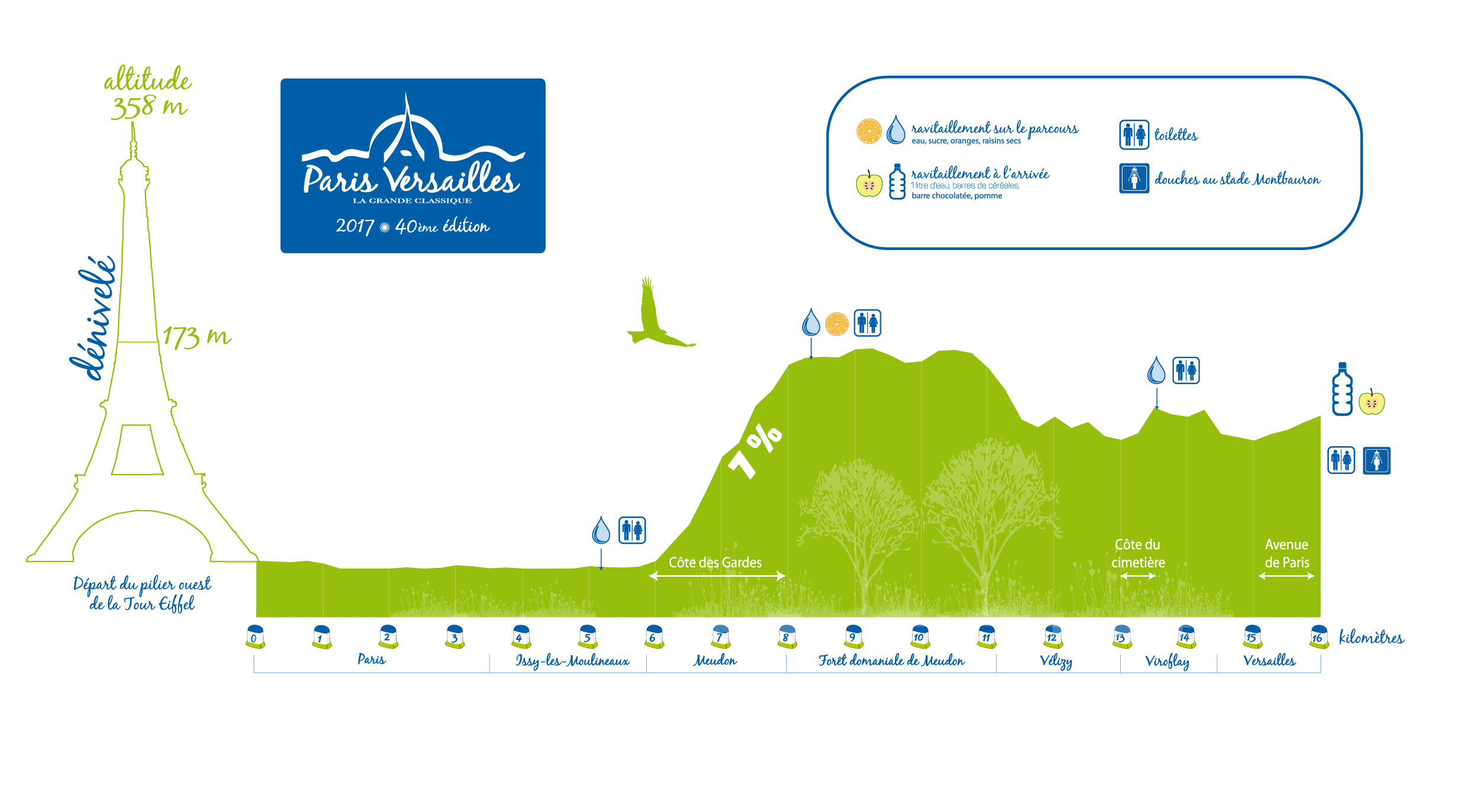 |
| The race profile |
So I started to wonder how could I improve my results for next year:
- If I grab 5 minutes next year, how will my ranking improve?
- Then, do I need to put my efforts in the first part or in the second part of the race?
Then I used interesting features in ggplot2 to elaborate space-time diagram to see how I was performing compared to my sibling runners. But it is not because I performed well (or not) that I made a good race... So what is a 'good' race?
Let start first with parsing the pdf file and tidying the resulting dataset.
library(pacman)
p_load("tabulizer")
p_load("magrittr", "dplyr", "tidyr","lubridate", "ggplot2", "reshape2")
location <- "http://www.parisversailles.com/docs/2017_resultats_provisoires.pdf"
liste <- extract_tables(location)
df <- as.data.frame(do.call(rbind, liste))
names(df) <- c("dossard", "nom", "prenom", "temps", "place", "categorie",
"hDepart", "hCotedesgardes", "hArrivee")
df %<>% mutate_all(funs(as.character(.))) %>% ungroup() %>%
filter(dossard != "Dossard" & prenom != "Prenom") #%>% select(-c("as.caracter(categorie)"))
Now let's add a bunch of new variables using the quite handy lubridate package.
options(digits.secs=2)
df %<>% mutate_at(c("hArrivee", "hDepart", "hCotedesgardes"),
funs(ymd_hms(paste0("2017-09-25 ",.)))) %>%
mutate(totalTime = difftime(hArrivee, hDepart, units="secs"),
halfTime = difftime(hCotedesgardes, hDepart, units="secs")) %>%
mutate(Rank = row_number(as.numeric(totalTime)),
partCotedesgardes = as.numeric(halfTime) / as.numeric(totalTime))
Last, I recalculate ranks (remember these where intermediate results and some runner where misclassified), ranks by category and finally add deciles
df %<>% group_by(categorie) %>% mutate(rankCat = row_number(Rank)) %>%
ungroup() %>% mutate(quant = cut(Rank, breaks = quantile(Rank, probs = seq(0, 1, 0.1),na.rm = TRUE), labels=1:10, right = TRUE, include.lowest=TRUE))
glimpse(df) Observations: 22,146 Variables: 15 $ dossard <chr> "18", "3", "25", "616", "43", "17", "11", "23", "699", "5", "37", "72... $ nom <chr> "GEDAMU", "GUIBAULT", "AZZAOUI", "RAUDIN", "LORRIAUX", "BETOUDJI", "G... $ prenom <chr> "Getinet", "Thierry", "Abdelmajid", "Stephane", "J-pierre", "Valentin... $ temps <chr> "00:52:50", "00:53:12", "00:54:48", "00:54:54", "00:54:58", "00:55:01... $ place <chr> "1", "2", "3", "4", "5", "6", "7", "8", "9", "10", "11", "12", "13", ... $ categorie <chr> "SH", "VH1", "SH", "SH", "VH1", "SH", "SH", "SH", "SH", "SH", "VH1", ... $ hDepart <dttm> 2017-09-25 09:59:57, 2017-09-25 09:59:57, 2017-09-25 09:59:57, 2017-... $ hCotedesgardes <dttm> 2017-09-25 10:26:45, 2017-09-25 10:26:45, 2017-09-25 10:27:05, 2017-... $ hArrivee <dttm> 2017-09-25 10:52:46, 2017-09-25 10:53:08, 2017-09-25 10:54:44, 2017-... $ totalTime <time> 3169.29 secs, 3191.89 secs, 3287.87 secs, 3293.73 secs, 3297.28 secs... $ halfTime <time> 1608.89 secs, 1608.73 secs, 1628.67 secs, 1665.71 secs, 1665.32 secs... $ Rank <int> 1, 2, 3, 4, 5, 6, 7, 8, 9, 10, 11, 12, 13, 14, 15, 16, 17, 18, 20, 19... $ partCotedesgardes <dbl> 0.5076500, 0.5040055, 0.4953572, 0.5057215, 0.5050587, 0.5043660, 0.5... $ rankCat <int> 1, 1, 2, 3, 2, 4, 5, 6, 7, 8, 3, 1, 9, 4, 10, 11, 12, 13, 15, 14, 16,... $ quant <fctr> 1, 1, 1, 1, 1, 1, 1, 1, 1, 1, 1, 1, 1, 1, 1, 1, 1, 1, 1, 1, 1, 1, 1,... | |
|
 |
| Arrival time of runners, my wife's position and mine (in secs) |
as.numeric(df$totalTime[df$dossard==armelle[1]]))
p <- df %>% mutate(totalTime = as.numeric(totalTime)) %>%
ggplot(aes(totalTime))+geom_density()
d <- ggplot_build(p)$data[[1]]
p + geom_segment(x=temps[1], xend=temps[1], y=0, yend=approx(x = d$x, y = d$y, xout = temps[1])$y, colour="red", size=1)+ geom_segment(x=temps[2], xend=temps[2], y=0, yend=approx(x = d$x, y = d$y, xout = temps[2])$y, colour="blue", size=1)
Interesting to notice, the best runner did it in 52 min, so an average of 18 km/h.
What if I want to run it 1h17 next time?
df %>% filter((totalTime >= 4620 & totalTime <= 4621) | dossard == 17421) %>%
summarise(ecartTemps=(max(totalTime)-min(totalTime))/60, ecartPlace = max(Rank)-min(Rank))
Well, I will grab 1889 ranks, out of 22132.
Now let's get back to my first question. How did I managed my race compared to my running siblings? By siblings I mean people whose performance were quite similar to mine. To do so, I slightly adapted the space-time graphic to reflect how I performed at the mid-point of the race, on top of this insane 7%-hill.
After a bit of scripting, melting,, casting my dataset (see reshape2) to fit it into the grammar of graphics, I get...
denis=c(17421, "Denis")
armelle=c(17422, "Armelle")
vincent=c(15845, "Vincent")
godefroy=c(21414, "Godefroy")
# Extraire les coureurs proche
k = denis
kTime = df %>% filter(dossard==k[1])%>%select(totalTime) %>% as.numeric()
df.tmp <- df %>% filter(totalTime >=(kTime-60) & totalTime <= (kTime+60)) %>%
mutate(starTime = 0) %>%
select(dossard, starTime, halfTime, totalTime)
df.tmp <- melt(df.tmp, id.vars = "dossard")
df.tmp %<>% mutate(x=ifelse(variable=="starTime",0, # convert x as numeric
ifelse(variable=="halfTime", 8, 16))) %>%
filter(!is.na(value)) %>% group_by(variable) %>% mutate(moy = mean(value)) %>%
ungroup() %>% mutate(ecart = value - moy)
df.tmp %>%
ggplot(aes(x, y=ecart, col=dossard), size=.2)+geom_line()+
theme(legend.position = 'none') +scale_color_grey() +
geom_line(data=subset(df.tmp, dossard==k[1]), aes(y=ecart), col="red")+
ggtitle(paste0("La course de ", k[2]))

Here is me, my girlfriend and my step-brother.
In the graph, you see the end-point race at 16 km, and the mid-point race at 8-km in x-axis.
Each line represent a runner and its deviation compared to the mean.
- A high point indicates a runner late at the midpoint (he took more time than others), but catching up quickly to finish with the same time as me.
- A low point indicates an early midpoint timing (the runner performed better than the others)

But does it make a 'good' race, and what is a 'good' race anyway?
Let see how the best runners compared to the others, using the percentage of running time spent during the first half of the race.

df %>% filter(dossard %in% c(17421, 17422, 21414))%>% select(dossard, partCotedesgardes, totalTime)
# A tibble: 3 x 3
dossard percentHalf totTime
 <chr>       <dbl>    <time>
21414    0.5000367 4219.77 s
17421    0.4908224 4883.09 s
17422 0.4974121 5481.29 s
I spent 49% of my race in the first half, and my brother-in-low 50%. Let see what this value is by decile.
df %>% filter(!is.na(partCotedesgardes)) %>%
     group_by(quant)%>%
     summarize(moy=mean(partCotedesgardes), sd=sd(partCotedesgardes))
# A tibble: 10 x 3
    quant       moy          sd
   <fctr>     <dbl>       <dbl>
 1      1 0.5022714 0.008330851
 2      2 0.5020689 0.010449567
 3      3 0.5010444 0.011329228
 4      4 0.4997301 0.012988530
 5      5 0.4991441 0.012154734
 6      6 0.4980548 0.013629279
 7      7 0.4963385 0.014371913
 8      8 0.4950229 0.015044514
 9      9 0.4914422 0.016621537
10     10 0.4880481 0.024609235
To this respect, I should have classified myself among the last decile!
I guess the explanation is that the best runners know how to weight their effort and keep some momentum, whereas the steep hill "kill" the others.